Geogrids under dynamic loading
Posted: 14 February 2006 | | No comments yet
The bearing performance of railway embankments on soft ground can be improved by high strength geosynthetic reinforcement products. Under operating conditions, the reinforcement is submitted to static and dynamic forces. The geosynthetic reinforcement products are made out of polymer materials, which show visco-elastic behaviour. Their long term deformation and strength depend on their creep behaviour under static loads and on their endurance properties under repeated cyclic traffic loads. In addition to short term tensile tests and creep tests, appropriate tests under cyclic loading have to be carried out in order to evaluate the long term response of geosynthetic reinforcement to dynamic actions.
The bearing performance of railway embankments on soft ground can be improved by high strength geosynthetic reinforcement products. Under operating conditions, the reinforcement is submitted to static and dynamic forces. The geosynthetic reinforcement products are made out of polymer materials, which show visco-elastic behaviour. Their long term deformation and strength depend on their creep behaviour under static loads and on their endurance properties under repeated cyclic traffic loads. In addition to short term tensile tests and creep tests, appropriate tests under cyclic loading have to be carried out in order to evaluate the long term response of geosynthetic reinforcement to dynamic actions.
The bearing performance of railway embankments on soft ground can be improved by high strength geosynthetic reinforcement products. Under operating conditions, the reinforcement is submitted to static and dynamic forces. The geosynthetic reinforcement products are made out of polymer materials, which show visco-elastic behaviour. Their long term deformation and strength depend on their creep behaviour under static loads and on their endurance properties under repeated cyclic traffic loads. In addition to short term tensile tests and creep tests, appropriate tests under cyclic loading have to be carried out in order to evaluate the long term response of geosynthetic reinforcement to dynamic actions.
The Munich-Augsburg railway line in Germany is one of the most heavily used trunk lines in Europe. Recently, in order to improve its capacity, two additional tracks were installed on the north side of the existing embankment. The new embankment section is founded on un-reinforced concrete columns and on stone columns which transmit the vertical loads through a soft organic clay layer to competent bearing ground (Figure 1). In order to limit the deformations of the embankment, to facilitate adequate serviceability as well as structural safety, the embankment is reinforced with four layers of knitted geogrids FORTRAC, composed of high-tenacity PET-yarns. The short term tensile strength of the two used geogrids employed here is 430 kN/m and 560 kN/m respectively in machine direction. Since the geogrid reinforcement is placed within a short distance below the rails, it experiences pronounced dynamic forces under passing trains. The performance of the geogrid under dynamic action was studied by specific cyclic load endurance testing.
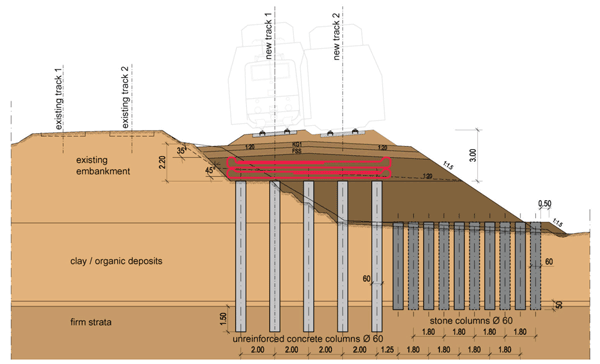

Figure 1: Railway embankment with Geogrid reinforcement
Basic arrangements have to be set for planning the performance of endurance tests for geogrids under different frequencies and loads. For the dimensioning of geogrid reinforced railroads it was fixed that the dynamic service loads have a sine shape. During the dynamic tests, sine loads were applied (Figure 2).
When a ‘Wöhler-curve’ is produced by endurance tests, as shown in Figure 2, then it is obvious that different components of the applied dynamic load can be varied stepwise. For such tests in the load controlled mode, it is mostly like a convention that the value of the stress or load ratio R is kept constant for all tests belonging to one individual ‘Wöhler-curve’. This statement seems to be trivial, but ‘Wöhler-curves’, for instance, with constant R and such ones with constant mean stress are very difficult to compare. Depending on the examined material, different shapes of ‘Wöhler-curves’ or fatigue curves may occur.
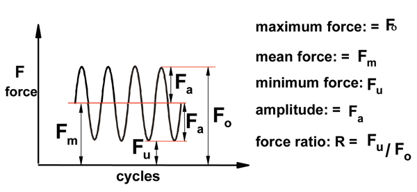

Figure 2: Nomenclature of the used symbols to specify the applied sine loads
In a half or double logarithmic plot, the classic ‘Wöhler-curve’ has the shape of curve 1 in Figure 3. There is a branch with load-depending limited life time followed by a branch parallel to the x-axis – the endurance limit where the break occurs is independent from the load. Many steels show such behaviour. Curve 2 has two branches with different slopes but no endurance limit. For instance, some aluminium alloys have this type of fatigue curve. Most of the thermoplastic materials show behaviour according to curve 3, or between curve 2 and 3. Thermoplastic materials show a more or less elastic-viscous behaviour; therefore an endurance limit like curve 1 can be excluded. In creep tests, these materials show a time-depending descent of strength. Under constant dynamic loading the estimated behaviour should be analogous Hellrich et al. 19791 and Schmiedel 19922. So the assumption of fatigue behaviour in accordance to curve 3 makes sense as it is conservative with respect to a later secure dimensioning of the geogrid. The final remark about Figure 3 is that curve 3 is only a straight line when either both axes are logarithmic or only the x-axis is logarithmic divided and additionally the corresponding regression function is applied.
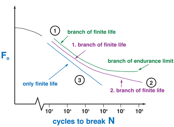

Figure 3: Schematic examples of 'Wöhler-curves'
The dynamic tests were performed in the load controlled mode in servo hydraulic machines. The strain was measured in the middle of each specimen. Additionally the specimen temperature was measured and reported. The set-up is shown in Figure 4.
Figure 4 shows that the specimen is clamped with capstan clamps. The hydraulic machines have a built in transducer for the piston stroke (not visible) and a load cell (shown at the top of Figure 4). These two signals plus the external ones from the extensometer and the thermocouples were reported and also used to compute online several derived functional values like the hysteresis, the loss and the stored work, the specimen stiffness and the amplitude of the extensometer stroke. Two series were performed. One series had a load frequency of 3 Hz and the other one had 10 Hz. In every series, 10 tests were placed on each of three verified load levels.
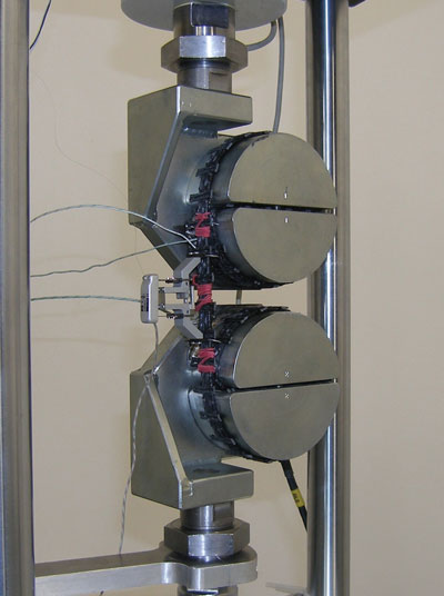

Figure 4: Test set-up for cyclic tests on geogrids
Due to the clamping, it can be expected that the process of material deterioration during the fatigue tests is controlled by multiple, non-additive effects. In such cases, the break events on every load level are mostly log-normal distributed. With this assumption the expected ‘Wöhler-curve’ has the appearance of a straight line in a double logarithmic plot. The ‘Wöhler-curve’ can be interpreted as line of 100% damage which is equal to the event break. During the dynamic loading, the material damage can start with the first cycle or with a later one. In the latter case there is, load depending, at the beginning a damage free specimen life followed by the life with accumulating damage until the break point is reached. This idea was formulated by Miner 19453. To quantify and to detect the damage, many researchers, e.g. Renz et al. 19864, have used the hysteresis and its properties because this is very sensitive. The curve marking the beginning of the damage is the limit line for 0% break or damage analogous to the limit line for the break events mentioned previously.
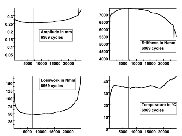

Figure 5: Detection of 'damage begin' by using synchronic moving curve cursor for different plots of test data
Due to the circumstance that the specimen fail earlier at 10 Hz loading than at 3 Hz, the following examples are given for 10 Hz test frequency. Figure 6 gives an example for the scatter of the break events for 10 Hz. For each load level the events were put into an order with increasing cycles to break and were logarithmised. After determining the mean or median value for each level, the data is ready to perform a regression to get the ‘Wöhler-line’, Figure 6. The tested geogrid has a short term tensile strength of 560 kN/m.
In the next step, a comfortable feature of our evaluation and presentation software was used to estimate the assumed ‘begin of damage’ for every complete test. Figure 5 shows four different plots for one test, where the x-axis performs unique cycles. In these plots there is a cursor which can be moved along one selected curve. The cursors in the other three plots follow the leading one in a synchronised motion. By using this feature special points can obviously be marked simultaneously.
Starting with the upper left plot in Figure 5, it shows the extensometer amplitude, and then the plot below shows the loss work. The lower right plot shows the temperature in the middle of the specimen and it is evident that the cursor marked local minima are corresponding with the local maximum of the stiffness in the upper right plot in Figure 5. This determination method was applied for all data sets. There were some gradual variations in the curve appearances; however, the main tendency was the same as stated for Figure 5. The received data for the ‘damage begin’ underwent the same evaluation procedure as reported for the break events. The fitting by the calculated regression lines is quite convincing and supports the assumption that there is a ‘damage begin’ and it shows that these events are reproducible and with a sufficient approximation log-normal distributed as well.
The last step of the evaluations is to put all points for the break events and for the assumed ‘damage begin’ in one lifetime diagram. This is shown in Figure 6. The upper function is the ‘Wöhler-line’ for 10 Hz test frequency and the line below represents the appertaining ‘damage begin’-line. Subsequently, the extrapolation of the geogrid life time under not explicit tested low loads delivers necessarily conservative results which can be used for further dimensioning purposes.
As stated before, tests with 3 Hz test frequency were also performed and analogue curves to Figure 6 were received. They were not presented here because they have less effect in terms of security dimensioning than those for 10 Hz. The ‘Wöhler line’ for 3 Hz lies over that of the 10 Hz. The same is valid for the pertaining ‘damage begin’-lines.
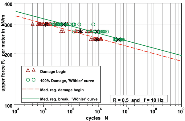

Figure 6: 'Wöhler-line' and the line for 'damage begin'
During 50 years service life, this railway structure is exposed to 108 cycles of traffic loading according to German Rail design practice. The design life of the structure is 120 years. In the case studied here, the design maximum tensile force of the geogrid reinforcement amounts to 60 kN/m. It can be seen in Figure 6 that for cyclic loading under the conditions of the tests reported here, the failure load at 108 cycles is much greater than the design load. So there is an adequate safety margin with respect to fatigue under dynamic loading.
References
- Hellrich, Harsch and Haenle (1979). Werkstoffführer Kunststoffe, Carl Hanser Verlag München, Wien 1979; ISBN 3-446-12662-7 (in German)
- Schmiedel, H. (1992). Handbuch der Kunststoffprüfung, Carl Hanser Verlag München, Wien 1992, ISBN 3-446-16336-0 (in German)
- Miner, M.A. (1945). Cumulative Damage in Fatigue, journal of appl. mech. trans. ASME 12, H.3, pp 154-164
- Renz, R., Altstätt, V. and Ehrenstein, G.W. (1986). “Hysteresis measurements for characterizing the dynamic fatigue of R-SMC”, 41st Conference Reinforced Plastic / Composite Institute, SPS, Atlanta 1986


